読む編集履歴表示

ハイゼンベルク描像

ウィキペディアから、無料の百科事典

ハイゼンベルク描像（はいぜんべるくびょうぞう、英: Heisenberg picture）またはハイゼンベルク表示（はいぜんべるくひょうじ、英: Heisenberg representation）は、物理学において量子力学を定式化するにあたり、演算子（可観測量やその他）が時間発展し、状態ベクトルは時間に依存しないとする理論形式のこと。状態ベクトルが時間発展し、演算子が時間に依存しないシュレーディンガー描像とは等価の結果を与える。

ハイゼンベルク力学とも呼ばれる行列力学は、時間発展にはハイゼンベルク描像を採用し、適当な基底を選んで演算子を行列表示したものに相当する。

相対論的な場の量子論では、ハイゼンベルク描像を採用するのが普通である^[1]。

数学的内容

ハイゼンベルク描像を採用する量子力学では、状態ベクトル $| ψ ⟩$ は時間発展せず、可観測量 $ˆ A (t)$ が下に示すハイゼンベルクの運動方程式に従い、時間発展する。

${\frac {\mathrm {d} }{\mathrm {d} t}}{\hat {A}}(t)={\frac {1}{i\hbar }}[{\hat {A}}(t),{\hat {H}}]+\left({\frac {\partial {\hat {A}}(t)}{\partial t}}\right)_{\text{classical}}.$

また、 $ˆ A (t)$ の期待値は以下で与えられる。

$\langle {\hat {A}}\rangle _{t}=\langle \psi |{\hat {A}}(t)|\psi \rangle .$

いくつかの意味で、ハイゼンベルク描像はシュレーディンガー描像より自然で、本質的だといえる。とくに、相対論的量子力学においてはローレンツ不変性はハイゼンベルク描像を用いてあらわされる。

また、古典力学との類似点が見やすいことも重要である。交換子をポアソン括弧で置き換えることによって、ハイゼンベルクの方程式はハミルトンの運動方程式と同じ形を与える。

ストーン-フォン・ノイマンの定理により、ハイゼンベルク描像とシュレーディンガー描像はユニタリ同値であることが示されている。

ハイゼンベルクの方程式とシュレーディンガー方程式の等価性

シュレーディンガー描像において、 $ˆ A$ を可観測量である(線形なエルミート演算子である)とすると、 $ˆ A$ のある状態 $| ψ ⟩$ における期待値は下のように求められる。

$\langle {\hat {A}}\rangle _{t}=\langle \psi (t)|{\hat {A}}|\psi (t)\rangle .$

また、シュレーディンガー方程式の形式解

$|\psi (t)\rangle =e^{-i{\hat {H}}t/\hbar }|\psi (0)\rangle$

を用いれば、物理量の期待値は、

$\langle {\hat {A}}\rangle _{t}=\langle \psi (0)|e^{i{\hat {H}}t/\hbar }{\hat {A}}e^{-i{\hat {H}}t/\hbar }|\psi (0)\rangle .$

よってハイゼンベルク描像において、状態は時間によらず常に $| ψ (0) ⟩$ であると定義し、物理量を表す演算子を次のように定義すれば、シュレーディンガー描像とハイゼンベルク描像とでは、物理量の期待値 $| ψ (t) ⟩$ は等しくなる。つまりシュレーディンガー描像とハイゼンベルク描像は時間発展について等価な理論になる。

${\hat {A}}(t):=e^{i{\hat {H}}t/\hbar }{\hat {A}}e^{-i{\hat {H}}t/\hbar }.$

すると $ˆ A (t)$ の時間依存性は、

${\begin{aligned}{\frac {\mathrm {d} }{\mathrm {d} t}}{\hat {A}}(t)&={\frac {i}{\hbar }}He^{i{\hat {H}}t/\hbar }{\hat {A}}e^{-i{\hat {H}}t/\hbar }+\left({\frac {\partial {\hat {A}}}{\partial t}}\right)_{\text{classical}}+{\frac {i}{\hbar }}e^{i{\hat {H}}t/\hbar }{\hat {A}}(-{\hat {H}})e^{-i{\hat {H}}t/\hbar }\\&={\frac {i}{\hbar }}e^{i{\hat {H}}t/\hbar }({\hat {H}}{\hat {A}}-{\hat {A}}{\hat {H}})e^{-i{\hat {H}}t/\hbar }+\left({\frac {\partial {\hat {A}}}{\partial t}}\right)_{\text{classical}}\\&={\frac {i}{\hbar }}({\hat {H}}{\hat {A}}(t)-{\hat {A}}(t){\hat {H}})+\left({\frac {\partial {\hat {A}}}{\partial t}}\right)_{\text{classical}}\\&={\frac {i}{\hbar }}[{\hat {H}},{\hat {A}}(t)]+\left({\frac {\partial {\hat {A}}}{\partial t}}\right)_{\text{classical}}.\end{aligned}}$

よってシュレーディンガー方程式から、次のハイゼンベルクの運動方程式が得られた。

${\mathrm {d} \over \mathrm {d} t}{\hat {A}}(t)={i \over \hbar }[{\hat {H}},{\hat {A}}(t)]+\left({\frac {\partial {\hat {A}}}{\partial t}}\right)_{\text{classical}}.$

関係式

${e^{\hat {B}}{\hat {A}}e^{-{\hat {B}}}}={\hat {A}}+[{\hat {B}},{\hat {A}}]+{\frac {1}{2!}}[{\hat {B}},[{\hat {B}},{\hat {A}}]]+{\frac {1}{3!}}[{\hat {B}},[{\hat {B}},[{\hat {B}},{\hat {A}}]]]+\cdots$

を使うと、時間依存な可観測量 $ˆ A (t)$ について下を得る。

${\hat {A}}(t)={\hat {A}}+{\frac {it}{\hbar }}[{\hat {H}},{\hat {A}}]-{\frac {t^{2}}{2!\hbar ^{2}}}[{\hat {H}},[{\hat {H}},{\hat {A}}]]-{\frac {it^{3}}{3!\hbar ^{3}}}[{\hat {H}},[{\hat {H}},[{\hat {H}},{\hat {A}}]]]+\cdots .$

交換子をポアソン括弧に置き換えると、この関係式は古典力学でも成り立つ。

交換関係

ハイゼンベルク描像では、演算子の時間依存性により、同時刻以外ではシュレーディンガー描像を用いたときと交換関係が異なる。例として、一次元調和振動子の $x (t 1), x (t 2), p (t 1), p (t 2)$ を考えてみると、系のハミルトニアンは

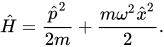
${\hat {H}}={\frac {{\hat {p}}^{2}}{2m}}+{\frac {m\omega ^{2}{\hat {x}}^{2}}{2}}.$

よって位置演算子と運動量演算子の時間発展は下のようになる。

${\mathrm {d} \over \mathrm {d} t}{\hat {x}}(t)={i \over \hbar }[{\hat {H}},{\hat {x}}(t)]={\frac {\hat {p}}{m}},$
${\mathrm {d} \over \mathrm {d} t}{\hat {p}}(t)={i \over \hbar }[{\hat {H}},{\hat {p}}(t)]=-m\omega ^{2}{\hat {x}}.$

これらをさらに時間微分し適当な初期条件

${\dot {\hat {p}}}(0)=-m\omega ^{2}{\hat {x}}(0),$
${\dot {\hat {x}}}(0)={\frac {{\hat {p}}(0)}{m}}$

を与えると下を得る。

${\hat {x}}(t)={\hat {x}}_{0}\cos(\omega t)+{\frac {{\hat {p}}_{0}}{\omega m}}\sin(\omega t),$
${\hat {p}}(t)={\hat {p}}_{0}\cos(\omega t)-m\omega {\hat {x}}_{0}\sin(\omega t).$

よって、直接交換関係を計算すると

$[{\hat {x}}(t_{1}),{\hat {x}}(t_{2})]={\frac {i\hbar }{m\omega }}\sin(\omega t_{2}-\omega t_{1}),$
$[{\hat {p}}(t_{1}),{\hat {p}}(t_{2})]=i\hbar m\omega \sin(\omega t_{2}-\omega t_{1}),$
$[{\hat {x}}(t_{1}),{\hat {p}}(t_{2})]=i\hbar \cos(\omega t_{2}-\omega t_{1}).$

同時刻 $t 1 = t 2$ においてはこの交換関係は正準交換関係に帰着することに注目すべきである。

脚注

↑ 清水明 2004.

参考文献

清水明『新版量子論の基礎―その本質のやさしい理解のために―』サイエンス社、2004年。ISBN 4-7819-1062-9。
Cohen-Tannoudji, Claude; Bernard Diu, Frank Laloe (1977). Quantum Mechanics (Volume One). Paris: Wiley. pp. 312-314. ISBN 047116433X

関連項目

表話編歴量子力学
全般	序論（英語版）数学的定式化
背景	古典力学前期量子論量子論量子力学の歴史量子力学の年表
基本概念	量子状態波動関数重ね合わせ不確定性原理可観測量相補性二重性不確定性トンネル効果排他原理エーレンフェストの定理量子もつれデコヒーレンス
定式化	シュレーディンガー描像ハイゼンベルク描像相互作用描像波動力学行列力学経路積分 GNS表現
方程式	シュレーディンガー方程式ハイゼンベルク方程式パウリ方程式クライン＝ゴルドン方程式ディラック方程式
実験	二重スリット実験シュテルン＝ゲルラッハの実験デイヴィソン＝ガーマーの実験ベルの不等式の検証実験（英語版）ポパーの実験（英語版）シュレーディンガーの猫爆弾検査問題（英語版）量子消しゴム実験
解釈（英語版）	観測問題ボーム解釈無矛盾歴史コペンハーゲン解釈アンサンブル解釈隠れた変数理論多世界解釈客観的収縮（英語版）量子論理関係性量子力学 (RQM)（英語版）確率過程量子化交流解釈（英語版）フォン・ノイマン＝ウィグナー解釈
人物	ジョン・スチュワート・ベルデヴィッド・ボームニールス・ボーアマックス・ボルンサティエンドラ・ボースルイ・ド・ブロイポール・ディラックポール・エーレンフェストヒュー・エヴェレット3世リチャード・P・ファインマンヴェルナー・ハイゼンベルクパスクアル・ヨルダンヘンリク・アンソニー・クラマースジョン・フォン・ノイマンヴォルフガング・パウリマックス・プランクエルヴィン・シュレーディンガーアルノルト・ゾンマーフェルトヴィルヘルム・ヴィーンユージン・ウィグナー
関連項目	散乱理論相対論的量子力学場の量子論量子情報量子カオス量子コンピューター
カテゴリ

この項目は、物理学に関連した書きかけの項目です。この項目を加筆・訂正などしてくださる協力者を求めています（プロジェクト:物理学／Portal:物理学）。